Tutorial 2: Antiferromagnetic State

In this tutorial, you will move beyond single-qubit control to explore Quantum Simulation. You will learn how to prepare an Antiferromagnetic (AFM) state, where atoms spontaneously arrange themselves in an alternating pattern: g - r - g - r.

1. The Physics: Adiabatic Evolution & Phase Transitions

Instead of using sharp pulses to flip qubits, we use a technique called Adiabatic Evolution.

Imagine a ball at the bottom of a valley. If you move the landscape very slowly, the ball will always stay at the bottom of the new valley. In quantum, the landscape is formed by the eigenvalues of the Ising Hamiltonian. The bottom of the valley is then the ground state of the Ising Hamiltonian, the state associated with the minimal eigenvalue. In quantum terms, if we change the time-dependent parameters of the Ising Hamiltonian slowly enough, the system of atoms should always be in the ground state ie state of minimal energy of the Ising Hamiltonian at a given time.

By varying the amplitude of the laser Ω and the laser frequency δ, we drive a phase transition that forces the atoms to reorganize from their initial state |gg…g⟩ into a checkerboard-like pattern to minimize their interaction energy (this is the AFM state).

2. Step-by-Step Implementation

1. Create a Register

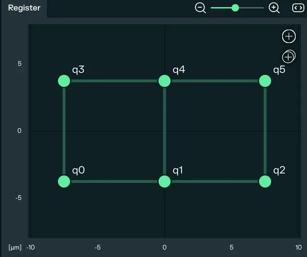
   A register is an arrangement of atoms in space. The positions of the atoms define the interaction energy between them, C₆/Rᵢⱼ⁶ (C6 is the Ising interaction coefficient, it depends on the principal quantum number of the Rydberg state, Rij is the distance between two atoms i and j). You can use the example from the example gallery or create your own register. After creating a new experiment, go to the Register tab. For this tutorial, we will use a 3x2 grid with an X and Y separation of 7.5 micrometers. Then click on Generate pattern.

   
   

2. Channel Selection For this simulation, we use the RYDBERG CHANNEL | GLOBAL just like in the Rabi oscillations tutorial. Since we want the entire register/array of atoms to evolve together, a global laser addressing all atoms is required.

   
   

   Removing the unused channels

   You can remove the unused channels by selecting them on the right panel and clicking on the remove channel button.

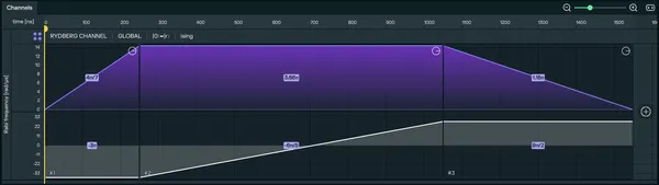
3. Design the Adiabatic Sequence Let’s implement a Sequence of pulses enabling to perform the preparation of the checkerboard state adiabatically. The Sequence will be composed of three pulses:

   • a first pulse over which the amplitude ramps up from 0 to a max amplitude, the detuning staying constant at -δ_off.
   • a second pulse over which the amplitude stays at max amplitude while the detuning ramps from -δ_off to δ_off.
   • a last pulse over which the amplitude ramps down to 0 while the detuning stays constant at δ_off.

   Here is how to implement it on pulser studio:

   Add the first pulse to the timeline by clicking the (+) button on the Rydberg Global row. Then, configure the pulse settings:

   • Amplitude Waveform: You should select Ramp to implement a linear sweep of the amplitude.
   • Detuning Waveform: You should select Constant to implement a constant detuning.
   • Both amplitude and detuning Duration: Set to 250 ns.
   • Detuning Value: Set to -12 π rad/µs. (You can play with it by clicking on the lock icon of the Area field)

   Zoom to fit

   You can update the view of the channels or the register by clicking on the Zoom to fit button on the top right of each panel.

   Add the second pulse to the timeline by clicking the (+) button on the Rydberg Global row. Then, configure the pulse settings:

   • Amplitude Waveform: You should select Constant to implement a constant amplitude. Why? Because we want to keep the amplitude constant to avoid saturation of the atoms.
   • Amplitude Value: Set to 4,6 π rad/µs.
   • Detuning Waveform: You should select Ramp to implement a linear sweep of the detuning.
   • Both amplitude and detuning Duration: Set to 800 ns.
   • Detuning Start Time: Set to -12 π rad/µs.
   • Detuning Stop Time: Set to 9 π rad/µs.

   Add the last pulse to the timeline by clicking the (+) button on the Rydberg Global row. Then, configure the pulse settings:

   • Amplitude Waveform: You should select Ramp.
   • Amplitude Start Time: Set to 4,6 π rad/µs.
   • Amplitude Stop Time: Set to 0 π rad/µs.
   • Detuning Waveform: You should select Constant to implement a constant detuning.
   • Both amplitude and detuning Duration: Set to 500 ns.
   • Detuning Value: Set to 9 π rad/µs.
   
   

4. Visualize and Run

   Now that you have designed the sequence, you should see the sequence in your timeline. You should be on the Local Emulation tab on the right panel, you can now press the Play button to run the simulation.

   You can also run the simulation on the cloud by clicking on the Cloud button on the top right of the panel.

   The cloud simulation will take longer to run than the local simulation, and you might have some different results.

   Go to the Simulation tab. Because we have multiple atoms, you will see the probability of the atoms being in the excited state.

   

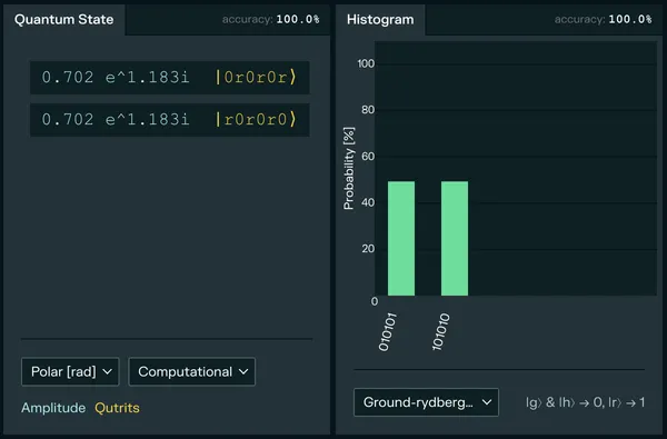
   The goal is to see a high probability for the states where no two adjacent atoms are both in the Rydberg state (e.g., the “checkerboard” pattern). This is the hallmark of the Antiferromagnetic order.

Interpreting Results

With multiple atoms, the results are more complex than in the Rabi tutorial. Here’s what to look for:

• The Checkerboard Pattern: Look for states with high probability where atoms alternate between 0 and r.
• The Rydberg Blockade at Scale: The reason neighbors don’t both excite to the Rydberg state “r” is the interaction energy (read more here). The system naturally evolves towards the AFM state because it is the lowest energy configuration (ground state of the final Ising Hamiltonian) under these conditions.

If you want to learn more about the theory of phase transitions with Rydberg atoms, you can read the Optimization tutorial in the Pulser documentation.